Generating biophysically detailed multi-compartmental models
This tutorial provides a walkthrough on how to use ISF in order to generate biophysically detailed multi-comparmental models that are consistent with empirical responses. To do this, you will need:
A neuron morphology in the
.hocformat.Empirical data on the neuron’s biophysical expression.
Empirical constraints on the electrophysiological response to input stimuli
These have been described in the previous tutorial.
ISF provides two ways of generating multi-compartmental neuron models:
Algorithm |
Pros |
Cons |
|
|---|---|---|---|
No a priori requirements |
Does not explore the full diversity of possible BDMs |
||
Explores the full biophysical diversity of possible BDMs |
Requires a seedpoint |
To get started, adapt your desired output path:
[1]:
from pathlib import Path
tutorial_output_dir = f"{Path.home()}/isf_tutorial_output" # <-- Change this to your desired output directory
[2]:
import Interface as I
%matplotlib inline
from getting_started import getting_started_dir
example_data_dir = I.os.path.join(getting_started_dir, 'example_data')
db = I.DataBase(tutorial_output_dir).create_sub_db("neuron_modeling")
model_db = I.DataBase(I.os.path.join(getting_started_dir, "example_data", "simulation_data", "biophysics"))
[INFO] ISF: Current version: heads/docs+0.gbb14e30d.dirty
[INFO] ISF: Current pid: 250365
[INFO] ISF: Loading mechanisms:
Warning: no DISPLAY environment variable.
--No graphics will be displayed.
[ATTENTION] ISF: The source folder has uncommited changes!
[INFO] ISF: Loaded modules with __version__ attribute are:
IPython: 8.12.2, Interface: heads/docs+0.gbb14e30d.dirty, PIL: 10.4.0, _brotli: 1.0.9, _csv: 1.0, _ctypes: 1.1.0, _curses: b'2.2', _decimal: 1.70, argparse: 1.1, backcall: 0.2.0, blosc: 1.11.1, bluepyopt: 1.9.126, brotli: 1.0.9, certifi: 2024.08.30, cffi: 1.17.0, charset_normalizer: 3.4.0, click: 7.1.2, cloudpickle: 3.1.0, colorama: 0.4.6, comm: 0.2.2, csv: 1.0, ctypes: 1.1.0, cycler: 0.12.1, cytoolz: 0.12.3, dash: 2.18.2, dask: 2.30.0, dateutil: 2.9.0, deap: 1.4, debugpy: 1.8.5, decimal: 1.70, decorator: 5.1.1, defusedxml: 0.7.1, distributed: 2.30.0, distutils: 3.8.20, django: 1.8.19, entrypoints: 0.4, executing: 2.1.0, fasteners: 0.17.3, flask: 1.1.4, fsspec: 2024.10.0, future: 1.0.0, greenlet: 3.1.1, idna: 3.10, ipaddress: 1.0, ipykernel: 6.29.5, ipywidgets: 8.1.5, isf_pandas_msgpack: 0.2.3, itsdangerous: 1.1.0, jedi: 0.19.1, jinja2: 2.11.3, joblib: 1.4.2, json: 2.0.9, jupyter_client: 7.3.4, jupyter_core: 5.7.2, kiwisolver: 1.4.5, logging: 0.5.1.2, markupsafe: 2.0.1, matplotlib: 3.5.1, msgpack: 1.0.8, neuron: 7.8.2+, numcodecs: 0.12.1, numexpr: 2.8.6, numpy: 1.19.2, packaging: 25.0, pandas: 1.1.3, parameters: 0.2.1, parso: 0.8.4, past: 1.0.0, pexpect: 4.9.0, pickleshare: 0.7.5, platform: 1.0.8, platformdirs: 4.3.6, plotly: 5.24.1, prompt_toolkit: 3.0.48, psutil: 6.0.0, ptyprocess: 0.7.0, pure_eval: 0.2.3, pydevd: 2.9.5, pygments: 2.18.0, pyparsing: 3.1.4, pytz: 2024.2, re: 2.2.1, requests: 2.32.3, scandir: 1.10.0, scipy: 1.5.2, seaborn: 0.12.2, six: 1.16.0, sklearn: 0.23.2, socketserver: 0.4, socks: 1.7.1, sortedcontainers: 2.4.0, stack_data: 0.6.2, statsmodels: 0.13.2, sumatra: 0.7.4, tables: 3.8.0, tblib: 3.0.0, tlz: 0.12.3, toolz: 1.0.0, tqdm: 4.67.1, traitlets: 5.14.3, urllib3: 2.2.3, wcwidth: 0.2.13, werkzeug: 1.0.1, yaml: 5.3.1, zarr: 2.15.0, zlib: 1.0, zmq: 26.2.0, zstandard: 0.19.0
Optimization Algorithm
This section will guide you through using ISF to create neuron models from scratch using a Multi-Objective Evolutionary Optimization algorithm (MOEA) called BluePyOpt.
Empirical limits for biophysical parameters
[3]:
from biophysics_fitting.hay.default_setup import get_feasible_model_params
params = get_feasible_model_params().drop('x', axis=1)
params.index = [e.replace('CaDynamics_E2', 'CaDynamics_E2_v2') for e in params.index]
params.index = 'ephys.' + params.index
In addition to the conductance of the ion channels, two important free parameters need to be added in order to find models for an L5PT:
The spatial distribution of \(SK_V3.1\) channels along the apical dendrite. These are modeled here to slope off from the soma towards the end of the apical dendrite, consistent with Schaefer et al. (2007)
The thickness of the apical dendrite. Why this is added as a free parameter is explained in this auxiliary notebook
[4]:
params = params.append(
I.pd.DataFrame({
'ephys.SKv3_1.apic.slope': {
'min': -3,
'max': 0
},
'ephys.SKv3_1.apic.offset': {
'min': 0,
'max': 1
}
}).T)
params = params.append(
I.pd.DataFrame({
'min': .333,
'max': 3
}, index=['scale_apical.scale']))
params = params.sort_index()
print("Empirical limits for biological parameters")
params
Empirical limits for biological parameters
[4]:
| min | max | |
|---|---|---|
| ephys.CaDynamics_E2_v2.apic.decay | 20.00000 | 200.00000 |
| ephys.CaDynamics_E2_v2.apic.gamma | 0.00050 | 0.05000 |
| ephys.CaDynamics_E2_v2.axon.decay | 20.00000 | 1000.00000 |
| ephys.CaDynamics_E2_v2.axon.gamma | 0.00050 | 0.05000 |
| ephys.CaDynamics_E2_v2.soma.decay | 20.00000 | 1000.00000 |
| ephys.CaDynamics_E2_v2.soma.gamma | 0.00050 | 0.05000 |
| ephys.Ca_HVA.apic.gCa_HVAbar | 0.00000 | 0.00500 |
| ephys.Ca_HVA.axon.gCa_HVAbar | 0.00000 | 0.00100 |
| ephys.Ca_HVA.soma.gCa_HVAbar | 0.00000 | 0.00100 |
| ephys.Ca_LVAst.apic.gCa_LVAstbar | 0.00000 | 0.20000 |
| ephys.Ca_LVAst.axon.gCa_LVAstbar | 0.00000 | 0.01000 |
| ephys.Ca_LVAst.soma.gCa_LVAstbar | 0.00000 | 0.01000 |
| ephys.Im.apic.gImbar | 0.00000 | 0.00100 |
| ephys.K_Pst.axon.gK_Pstbar | 0.00000 | 1.00000 |
| ephys.K_Pst.soma.gK_Pstbar | 0.00000 | 1.00000 |
| ephys.K_Tst.axon.gK_Tstbar | 0.00000 | 0.10000 |
| ephys.K_Tst.soma.gK_Tstbar | 0.00000 | 0.10000 |
| ephys.NaTa_t.apic.gNaTa_tbar | 0.00000 | 0.04000 |
| ephys.NaTa_t.axon.gNaTa_tbar | 0.00000 | 4.00000 |
| ephys.NaTa_t.soma.gNaTa_tbar | 0.00000 | 4.00000 |
| ephys.Nap_Et2.axon.gNap_Et2bar | 0.00000 | 0.01000 |
| ephys.Nap_Et2.soma.gNap_Et2bar | 0.00000 | 0.01000 |
| ephys.SK_E2.apic.gSK_E2bar | 0.00000 | 0.01000 |
| ephys.SK_E2.axon.gSK_E2bar | 0.00000 | 0.10000 |
| ephys.SK_E2.soma.gSK_E2bar | 0.00000 | 0.10000 |
| ephys.SKv3_1.apic.gSKv3_1bar | 0.00000 | 0.04000 |
| ephys.SKv3_1.apic.offset | 0.00000 | 1.00000 |
| ephys.SKv3_1.apic.slope | -3.00000 | 0.00000 |
| ephys.SKv3_1.axon.gSKv3_1bar | 0.00000 | 2.00000 |
| ephys.SKv3_1.soma.gSKv3_1bar | 0.00000 | 2.00000 |
| ephys.none.apic.g_pas | 0.00003 | 0.00010 |
| ephys.none.axon.g_pas | 0.00002 | 0.00005 |
| ephys.none.dend.g_pas | 0.00003 | 0.00010 |
| ephys.none.soma.g_pas | 0.00002 | 0.00005 |
| scale_apical.scale | 0.33300 | 3.00000 |
Database setup
The MOEA algorithm expects a database containing methods that set up Simulator and Evaluator objects. Let’s create these methods. Here, you can set up which input stimuli will be run, and how they will be evaluated. We have already created such simulation setup and evaluation methods for L5PTs consistent with Hay et al. (2011) in default_setup and L5tt_parameter_setup
[5]:
from biophysics_fitting.L5tt_parameter_setup import get_L5tt_template_v2
import biophysics_fitting.hay.default_setup as hay_setup
def scale_apical(cell_param, params):
assert(len(params) == 1)
cell_param.cell_modify_functions.scale_apical.scale = params['scale']
return cell_param
def get_fixed_params(db_setup):
"""
Configure the fixed params and return
"""
fixed_params = db_setup['fixed_params']
fixed_params['morphology.filename'] = db_setup['morphology'].get_file(
'hoc')
return fixed_params
def get_Simulator(db_setup, step=False):
"""
Configure the Simulator object and return
"""
fixed_params = db_setup['get_fixed_params'](db_setup)
s = hay_setup.get_Simulator(
I.pd.Series(fixed_params),
step=step)
s.setup.cell_param_generator = get_L5tt_template_v2
s.setup.cell_param_modify_funs.append(
('scale_apical', scale_apical)
)
s.setup.params_modify_funs_after_cell_generation = []
return s
def get_Evaluator(db_setup, step=False):
"""
No additional configuration is needed for the Evaluator, simply return biophysics_fitting.L5tt_parameter_setup.get_Evaluator
"""
return hay_setup.get_Evaluator(step=step)
def get_Combiner(db_setup, step=False):
"""
No additional configuration is needed for the Combiner, simply return biophysics_fitting.L5tt_parameter_setup.get_Combiner
"""
return hay_setup.get_Combiner(step=step)
Now, the database for optimization can be set up as seen below.
[6]:
def set_up_db_for_MOEA(db, morphology_id='89', morphology="", step=False):
"""
Set up a DataBase for MOEA.
Args:
db: a DataBase object
morphology_id: name of the morphology
morphology: path to a .hoc morphology file
step: whether or not to perform step current injections
Returns:
data_base.DataBase: a database containing:
- fixed_params
- get_fixed_params
- get_Simulator
- get_Evaluator
- get_Combiner
- the morphology file
"""
from data_base.IO.LoaderDumper import pandas_to_pickle, to_cloudpickle
db.create_sub_db(morphology_id)
db[morphology_id].create_managed_folder('morphology')
I.shutil.copy(
I.os.path.join(
morphology
), db[morphology_id]['morphology'].join(
morphology.split(I.os.sep)[-1]
))
db[morphology_id]['fixed_params'] = {
'BAC.hay_measure.recSite': 294.8203371921156, # recording site on the apical dendrite for BAC
'BAC.stim.dist': 294.8203371921156, # stimulus injection site on the apical dendrite for BAC
'bAP.hay_measure.recSite1': 294.8203371921156, # recording site 1 on the apical dendrite for bAP
'bAP.hay_measure.recSite2': 474.8203371921156, # recording site 2 on the apical dendrite for bAP
'hot_zone.min_': 384.8203371921156, # calcium zone start
'hot_zone.max_': 584.8203371921156, # calcium zone end
'hot_zone.outsidescale_sections': [23,24,25,26,27,28,29,31,32,33,34,35,37,38,40,42,43,44,46,48,50,51,52,54,56,58,60],
'morphology.filename': None
}
db[morphology_id]['get_fixed_params'] = get_fixed_params
db[morphology_id].set('params', params, dumper=pandas_to_pickle)
db[morphology_id].set('get_Simulator',
I.partial(get_Simulator, step=step),
dumper=to_cloudpickle)
db[morphology_id].set('get_Evaluator',
I.partial(get_Evaluator, step=step),
dumper=to_cloudpickle)
db[morphology_id].set('get_Combiner',
I.partial(get_Combiner, step=step),
dumper=to_cloudpickle)
return db
Let’s copy over a morphology and initialize our DataBase for the optimization run
[7]:
morphology_id = "89"
morphology_path = I.os.path.join(
example_data_dir,
"anatomical_constraints",
"89_C2.hoc")
[8]:
if "morphology" in db[morphology_id].keys():
# In case you are re-running this tutorial
del db[morphology_id]["morphology"]
[9]:
db = set_up_db_for_MOEA(
db,
morphology_id="89",
morphology=morphology_path,
step=False
)
db.ls(max_lines_per_key=10)
[WARNING] isf_data_base: The database source folder has uncommitted changes!
[WARNING] isf_data_base: The database source folder has uncommitted changes!
[WARNING] isf_data_base: The database source folder has uncommitted changes!
[WARNING] isf_data_base: The database source folder has uncommitted changes!
[WARNING] isf_data_base: The database source folder has uncommitted changes!
[WARNING] isf_data_base: The database source folder has uncommitted changes!
[WARNING] isf_data_base: The database source folder has uncommitted changes!
<data_base.isf_data_base.isf_data_base.ISFDataBase object at 0x2b6ac67a19a0>
Located at /gpfs/soma_fs/home/meulemeester/isf_tutorial_output/neuron_modeling/db
db
├── voltage_traces
├── burst_trail_video
├── burst_trail_ca_current_video
├── images
├── simulator
├── burst_trail_video_3d
├── Ca_LVAst_video_3d
└── 89
├── params
├── get_Simulator
├── morphology
├── get_fixed_params
├── RW_exploration_example
├── fixed_params
├── get_Evaluator
├── get_Combiner
└── 42/...
Run the optimization algorithm
We’re now ready to run the optimization algorithm.
[10]:
seedpoint = 42
if str(seedpoint) in db[morphology_id].keys():
# In case you are re-running this tutorial
del db[morphology_id][str(seedpoint)]
[11]:
population = I.bfit_start_run(
db['89'],
n=seedpoint,
client=I.get_client(),
offspring_size=10, # Low amount of offspring just as an example
pop=None, # adapt this to the output population of the previous run to continue where you left off
continue_cp=False, # If you want to continue a preivoius run, set to True
max_ngen=1 # run for just 1 generation
)
[WARNING] isf_data_base: The database source folder has uncommitted changes!
[WARNING] isf_data_base: The database source folder has uncommitted changes!
[WARNING] isf_data_base: The database source folder has uncommitted changes!
starting multi objective optimization with 5 objectives and 35 parameters
[WARNING] isf_data_base: The database source folder has uncommitted changes!
The results are written out after each generation. We have an offspring size of \(10\), so we will find \(10\) proposed biophysical models in generation \(1\) of our seedpoint.
Inspecting the optimizer results
As the optimization algorithm did not run for very long, they likely will not produce very good results:
[12]:
population = db['89'][str(seedpoint)]['1']
objectives = population.drop(params.index, axis=1)
objectives
[12]:
| BAC_APheight.check_1AP | BAC_APheight.raw | BAC_APheight.normalized | BAC_APheight | BAC_ISI.check_2_or_3_APs | BAC_ISI.check_repolarization | BAC_ISI.raw | BAC_ISI.normalized | BAC_ISI | BAC_caSpike_height.check_1_Ca_AP | ... | bAP_att3.check_1_AP | bAP_att3.check_relative_height | bAP_att3.normalized | bAP_att3 | bAP.err | bAP.check_minspikenum | bAP.check_returning_to_rest | bAP.check_no_spike_before_stimulus | bAP.check_last_spike_before_deadline | bAP.check_max_prestim_dendrite_depo | |
|---|---|---|---|---|---|---|---|---|---|---|---|---|---|---|---|---|---|---|---|---|---|
| 0 | True | [] | NaN | 247.723719 | False | True | NaN | NaN | 247.723719 | False | ... | False | True | 3.247603 | 249.664128 | 249.664128 | False | True | True | True | NaN |
| 1 | True | [37.86503410206352] | 2.573007 | 243.919564 | False | True | NaN | NaN | 243.919564 | False | ... | True | True | 2.995773 | 2.995773 | 249.537994 | True | True | True | True | NaN |
| 2 | True | [] | NaN | 246.651239 | False | True | NaN | NaN | 246.651239 | True | ... | False | True | 3.158216 | 249.546677 | 249.546677 | False | True | True | True | NaN |
| 3 | True | [0.18474967506085127] | 4.963050 | 244.294466 | False | True | NaN | NaN | 244.294466 | True | ... | True | True | 1.793552 | 1.793552 | 249.348300 | True | True | True | True | NaN |
| 4 | True | [] | NaN | 249.131673 | False | True | NaN | NaN | 249.131673 | False | ... | False | True | 3.331860 | 249.880194 | 249.880194 | False | True | True | True | NaN |
| 5 | True | [] | NaN | 249.247658 | False | True | NaN | NaN | 249.247658 | False | ... | False | True | 3.329374 | 249.915740 | 249.915740 | False | True | True | True | NaN |
| 6 | True | [42.48873193409531] | 3.497746 | 242.681292 | False | True | NaN | NaN | 242.681292 | True | ... | True | True | 5.466243 | 5.466243 | 249.452332 | True | True | True | True | NaN |
| 7 | True | [] | NaN | 248.397994 | False | True | NaN | NaN | 248.397994 | False | ... | False | True | 3.223281 | 249.805852 | 249.805852 | False | True | True | True | NaN |
| 8 | True | [] | NaN | 249.099842 | False | True | NaN | NaN | 249.099842 | False | ... | False | True | 3.330868 | 249.873099 | 249.873099 | False | True | True | True | NaN |
| 9 | True | [] | NaN | 247.422501 | False | True | NaN | NaN | 247.422501 | False | ... | False | True | 3.208826 | 249.675405 | 249.675405 | False | True | True | True | NaN |
10 rows × 59 columns
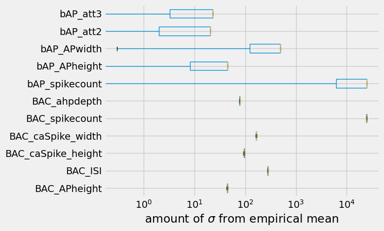
Most values are about \(250 \sigma\) removed from the empirical mean. this is a default fill value for voltage traces that flatline. Howver, voltage traces that exhibit some variance are penalized slightly less compared to those that completely do nothing. Some other objectives are already quite close! What is the spread on the empirical data?
[13]:
from biophysics_fitting.hay.default_setup import get_hay_problem_description
objectives_std = [ # the empirical objectives in units of standard deviation from the mean
e for e in objectives.columns
if not any(
[tag in e
for tag in (".raw", ".normalized", "check", ".err")
])
]
empirical_data = get_hay_problem_description()
empirical_data = empirical_data[empirical_data['objective'] \
.isin(objectives_std)] \
.set_index("objective") \
.loc[objectives_std]
print("Empirical distribution for physiology objectives")
empirical_data
Empirical distribution for physiology objectives
[13]:
| feature | mean | std | stim_name | stim_type | |
|---|---|---|---|---|---|
| objective | |||||
| BAC_APheight | AP_height | 25.000 | 5.0000 | BAC | BAC |
| BAC_ISI | BAC_ISI | 9.901 | 0.8517 | BAC | BAC |
| BAC_caSpike_height | BAC_caSpike_height | 6.730 | 2.5400 | BAC | BAC |
| BAC_caSpike_width | BAC_caSpike_width | 37.430 | 1.2700 | BAC | BAC |
| BAC_spikecount | Spikecount | 3.000 | 0.0100 | BAC | BAC |
| BAC_ahpdepth | AHP_depth_abs | -65.000 | 4.0000 | BAC | BAC |
| bAP_spikecount | Spikecount | 1.000 | 0.0100 | bAP | bAP |
| bAP_APheight | AP_height | 25.000 | 5.0000 | bAP | bAP |
| bAP_APwidth | AP_width | 2.000 | 0.5000 | bAP | bAP |
| bAP_att2 | BPAPatt2 | 45.000 | 10.0000 | bAP | bAP |
| bAP_att3 | BPAPatt3 | 36.000 | 9.3300 | bAP | bAP |
So \(250\ \sigma\) is obviously quite far away from the empirical data. Then again, the model did not run for very long. In general, the initial models proposed by the evolutionary algorithm do not do reproduce empirically observed responses, and are quite far off. It takes a lot more than an offspring size of \(10\) and a single generation to get close to a model that reproduces empirically observed responses.
To finalize the optimization, let’s see how many of the objectives got close to the empirical mean.
[14]:
I.plt.style.use("fivethirtyeight")
diff = (objectives[objectives_std] - empirical_data['mean']) / empirical_data["std"]
ax = diff.plot.box(vert=False)
ax.set_xscale('log')
ax.set_xlabel("amount of $\sigma$ from empirical mean")
[14]:
Text(0.5, 0, 'amount of $\\sigma$ from empirical mean')
See the previous tutorial for more information on how to evaluate biophysically detailed single-cell models.
Exploration from seedpoint
Assuming that we have a biophysical model that performs well on all objectives, it is possible to continuously make variations on the biophysical parameters while keeping the objectives in-distribution.
This is conveniently packaged in biophysics_fitting.exploration_from_seedpoint.
[15]:
if not I.os.path.exists(I.os.path.join(db["89"].basedir, 'RW_exploration_example')):
db["89"].create_managed_folder('RW_exploration_example')
We provide some working models for this morphology below.
[16]:
model_db["example_models"]
[16]:
| ephys.CaDynamics_E2_v2.apic.decay | ephys.CaDynamics_E2_v2.apic.gamma | ephys.CaDynamics_E2_v2.axon.decay | ephys.CaDynamics_E2_v2.axon.gamma | ephys.CaDynamics_E2_v2.soma.decay | ephys.CaDynamics_E2_v2.soma.gamma | ephys.Ca_HVA.apic.gCa_HVAbar | ephys.Ca_HVA.axon.gCa_HVAbar | ephys.Ca_HVA.soma.gCa_HVAbar | ephys.Ca_LVAst.apic.gCa_LVAstbar | ... | BAC_bifurcation_charges.Ca_LVAst.ica | BAC_bifurcation_charges.SKv3_1.ik | BAC_bifurcation_charges.Ca_HVA.ica | BAC_bifurcation_charges.Ih.ihcn | BAC_bifurcation_charges.NaTa_t.ina | BAC_bifurcation_charge | inside | n_suggestion | iteration | particle_id | |
|---|---|---|---|---|---|---|---|---|---|---|---|---|---|---|---|---|---|---|---|---|---|
| 0 | 30.136941 | 0.004712 | 281.483947 | 0.002268 | 90.694969 | 0.022993 | 0.000006 | 0.000664 | 0.000443 | 0.172148 | ... | 2.327926 | 0.125072 | 0.008035 | 0.008034 | 0.076292 | 2.558079 | True | NaN | 0 | 0 |
| 12 | 30.090741 | 0.004497 | 281.461630 | 0.002050 | 91.323819 | 0.023132 | 0.000022 | 0.000668 | 0.000445 | 0.171266 | ... | 2.347116 | 0.146069 | 0.032371 | 0.008043 | 0.078511 | 2.624398 | True | 2.0 | 12 | 0 |
| 14 | 31.140835 | 0.004243 | 280.558319 | 0.002085 | 97.416916 | 0.023266 | 0.000044 | 0.000671 | 0.000443 | 0.171614 | ... | 2.367618 | 0.149355 | 0.063454 | 0.008050 | 0.075175 | 2.791949 | True | 1.0 | 14 | 0 |
| 40 | 30.040827 | 0.004158 | 281.350880 | 0.002013 | 92.144582 | 0.022963 | 0.000073 | 0.000671 | 0.000444 | 0.172023 | ... | 2.342807 | 0.116513 | 0.108821 | 0.007992 | 0.075548 | 2.811305 | True | 2.0 | 40 | 0 |
| 56 | 29.865605 | 0.003981 | 282.074662 | 0.001969 | 94.770400 | 0.022873 | 0.000095 | 0.000665 | 0.000447 | 0.171751 | ... | 2.301322 | 0.043190 | 0.147240 | 0.007872 | 0.082982 | 2.670060 | True | 1.0 | 56 | 0 |
5 rows × 399 columns
Setup the random walk exploration
there are many different kinds of exploration one could do. We will simply use a random walk, as it has proven to be both efficient and capable of broadly sampling the bipohysical parameter space.
[17]:
evaluator = db["89"]["get_Evaluator"](db['89'])
simulator = db["89"]["get_Simulator"](db['89'])
biophysical_parameter_ranges = db['89']['params']
example_models = model_db['example_models']
biophysical_parameter_names = [e for e in example_models.columns if "ephys" in e or e == "scale_apical.scale"]
[18]:
from biophysics_fitting.exploration_from_seedpoint.RW import RW
from biophysics_fitting.exploration_from_seedpoint.utils import evaluation_function_incremental_helper
from biophysics_fitting.hay.evaluation import hay_evaluate_bAP, hay_evaluate_BAC
evaluation_function = I.partial(
evaluation_function_incremental_helper, # this incremental helper stops the evaluation as soon as a stimulus protocol doesn't work.
s=simulator,
e=evaluator,
stim_order=['bAP', 'BAC']
)
rw = RW(
param_ranges = biophysical_parameter_ranges,
df_seeds = example_models[biophysical_parameter_names],
evaluation_function = evaluation_function,
MAIN_DIRECTORY = db["89"]['RW_exploration_example'],
min_step_size = 0.02,
max_step_size = 0.02,
checkpoint_every = 1 # This is a lot of IO. Increase this value if you are not merely doing an example.
)
Run the exploration algorithm
Let’s run this for 10 seconds. You can always restart the exploration and it will pick up from where it left off. If you are not running this on High-Performance Computing, you may want to increase the duration.
[19]:
duration = 10 # in seconds
from time import sleep
from threading import Thread
import multiprocessing
proc = multiprocessing.Process(
target=rw.run_RW,
kwargs={
'selected_seedpoint': 0,
'particle_id': 0,
'seed': 42 # for numpy random seed
})
# --- run for some time, then kill the process
proc.start()
sleep(duration)
proc.terminate() # sends a SIGTERM
proc.join()
evaluating stimulus bAP
evaluating stimulus BAC
all stimuli successful!
evaluating stimulus bAP
evaluating stimulus BAC
all stimuli successful!
evaluating stimulus bAP
evaluating stimulus BAC
all stimuli successful!
evaluating stimulus bAP
[20]:
from biophysics_fitting.exploration_from_seedpoint.RW_analysis import Load
outdir = db["89"]['RW_exploration_example'].join('0')
l = Load(
client=I.get_client(),
path=outdir,
n_particles = 1)
[21]:
explored_models = l.get_df().compute()
print("Explored {} new models".format(len(explored_models)))
Explored 14 new models
Inspecting the exploration results
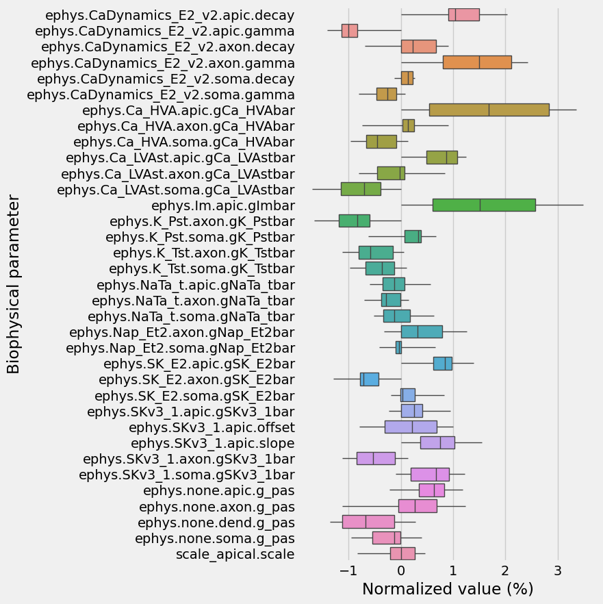
How much did the exploration actually explore? Let’s plot out how much it deviated from it’s starting point, relative to the total extent of parameter limits we allowed for
[22]:
def normalize(df, mn, mx):
return (df - mn)/(mx-mn)
mn, mx = biophysical_parameter_ranges['min'], biophysical_parameter_ranges['max']
normalized_startpoint = normalize(example_models.iloc[0][biophysical_parameter_names], mn, mx)
normalized_explored_models = normalize(explored_models[biophysical_parameter_names], mn, mx)
# calc exploration relative to startpoint, in % of total allowed parameter limits
d = I.pd.concat([normalized_explored_models, I.pd.DataFrame(normalized_startpoint).T])
d -= normalized_startpoint
d[biophysical_parameter_names] *= 100
d = d.melt(var_name='Biophysical parameter', value_name='Normalized value (%)')
[23]:
I.plt.figure(figsize=(5, 10))
ax = I.sns.boxplot(
data=d,
y='Biophysical parameter', x='Normalized value (%)',
whis=100,
linewidth=1,
showcaps = False
)
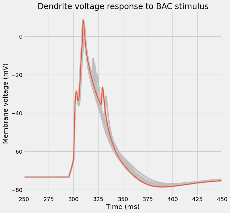
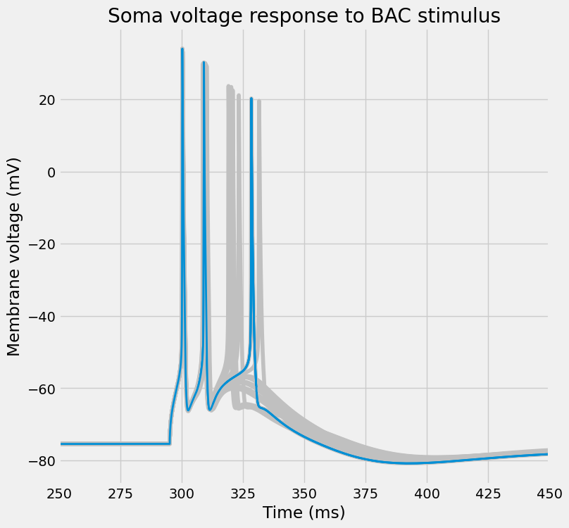
Let’s check what the resulting voltage traces look like
[24]:
delayeds = [
I.dask.delayed(simulator.run)(p, 'BAC')
for _, p in explored_models[biophysical_parameter_names].iterrows()
]
f = I.get_client().compute(delayeds)
[25]:
responses = [f_.result() for f_ in f]
BAC_responses = [response['BAC.hay_measure'] for response in responses]
[26]:
soma_voltages = [
e['vList'][0] for e in BAC_responses
]
dend_voltages = [
e['vList'][1] for e in BAC_responses
]
time_points = [
e['tVec'] for e in BAC_responses
]
[27]:
def plot_traces(ax, time_points, voltages, highlight_id, color, title):
for t, v in zip(time_points, voltages):
ax.plot(t, v, c="silver")
ax.plot(
time_points[highlight_id],
voltages[highlight_id],
c=color,
lw=2
)
ax.set_title(title)
ax.set_xlabel("Time (ms)")
ax.set_ylabel("Membrane voltage (mV)")
ax.set_xlim(250, 450)
[28]:
colors = I.plt.rcParams['axes.prop_cycle'].by_key()['color']
random_model = I.np.random.randint(0, len(BAC_responses))
print("Highlighting model nr. {}".format(random_model))
Highlighting model nr. 11
[29]:
fig, ax = I.plt.subplots(1, 1, figsize=(8, 8))
plot_traces(
ax,
time_points,
dend_voltages,
random_model,
colors[1],
title="Dendrite voltage response to BAC stimulus"
)
[30]:
fig, ax = I.plt.subplots(1, 1, figsize=(8, 8))
plot_traces(
ax,
time_points,
soma_voltages,
random_model,
colors[0],
title="Soma voltage response to BAC stimulus"
)
Or, per usual, visualize the entire dendritic tree.
[31]:
cell, _ = simulator.get_simulated_cell(
explored_models[biophysical_parameter_names].iloc[random_model],
"BAC")
[32]:
from visualize.cell_morphology_visualizer import CellMorphologyVisualizer as CMV
CMV(
cell,
t_start=250,
t_stop=400,
t_step=1,
).animation(
images_path=db.basedir+'/images',
color="voltage",
client=I.get_client(),
show_legend=True
)
Recap
The sections above have described how to use ISFs modeling capabilities (the Simulator and Evaluator) to produce bipohysically detailed multi-compartmental neuron models, using nothing but:
A neuron morphology in the
.hocformat.Empirical data on the neuron’s biophysical expression.
Empirical constraints on the electrophysiological response to input stimuli
This approach effectively allows you to explore a broad and diverse range of neuron models, all o fhwich capture the intrinsic physiology of the neuron.